
Bayesian Statistics, Maximum Likelihood Estimation, and Machine Learning
Resources
- Wikipedia: Prior Probability
- Wikipedia: Posterior Probability
- Wikipedia: Maximum Likelihood Estimation
- Youtube: 오토인코더의 모든 것 1/3
Prior probability
The prior probability distribution of an uncertain quantity is the probability distribution about that quantity before some evidence is taken into account. This is often expressed as \(p(\theta)\).
Posterior probability
The posterior probability of a random event is the conditional probability that is assigned after relevant evidence is taken into account. This is often expressed as \(p(\theta | X)\). The prior and posterior probabilities are related by the Bayes’ Theorem as follows:
\[p(\theta | x) = \frac{p(x|\theta)p(\theta)}{p(x)}\]Maximum Likelihood Estimation (MLE)
MLE is a method of estimating the parameters of a statistical model, given observations. Intuitively, we are trying to find the model parameters that make the observed data most probable. This is done by finding the parameters that maximizes the likelihood function \(\mathcal{L}(\theta;x)\). When we are dealing with discrete random variables, the likelihood function is the probability. On the other hand, when we are dealing with continuous random variables, the likelihood function is the value of the probability distribution function.
We can formulate the MLE problem as follows:
\[\theta^* \in \{\underset{\theta}{\text{argmax}} \mathcal{L}(\theta;x)\}\]where \(\theta\) is the model parameters and \(x\) is the observed data.
We often use the average log-likelihood function
\[\hat{\mathcal{l}}(\theta;x) = \frac{1}{n} \log \mathcal{L}(\theta;x)\]since it has preferable qualities. One of this is illustrated later in this document.
Machine Learning in the MLE perspective
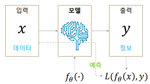
A traditional machine learning model for classification is visualized as the above: we receive an input image \(x\) and our model calculates \(f_\theta (x)\), which is a vector denoting the probability for each class. Then based on our label, we calculate the loss function, which is then optimized using gradient descent. Now, let us view this in a maximum likelihood perspective.
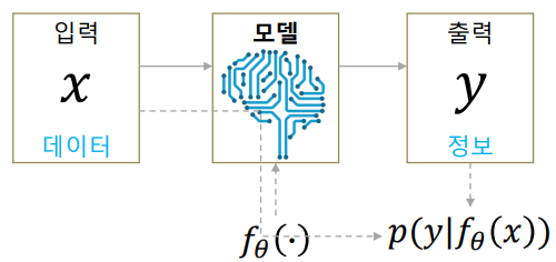
Now, when we create an ML model, we choose a statistical model that our output may follow. Then, our ML model function calculates the parameters of that statistical model. For example, let us assume that our output \(y\) is one dimensional and has a Gaussian distribution. Then we set \(f_\theta(x)\) to a two-dimensional vector and interpret it as
\[f_\theta(x) =\begin{bmatrix}\mu\\\sigma\end{bmatrix}\]Thus for each input \(x\) we obtain a Gaussian distribution for \(y\). Using negative log-likelihood, our optimization problem is the following:
\[\theta^* = \underset{\theta}{\text{argmin}}[-\log p(y|f_\theta(x))]\]If we assume that our inputs are independent and identically distributed (i.i.d), we can obtain the following:
\[p(y|f_\theta(x)) = \prod_i p(y_i|f_\theta(x_i))\]Rewriting our optimization problem:
\[\theta^* = \underset{\theta}{\text{argmin}}[-\sum_i\log p(y_i|f_\theta(x_i))]\]When we perform inference from our model, we no longer get determined outputs as we did in traditional machine learning models. We now get a distribution of \(y_\text{new}\),
\[y_\text{new} \sim f_{\theta^*}(x_\text{new})\]where we should sample a single \(y_\text{new}\).
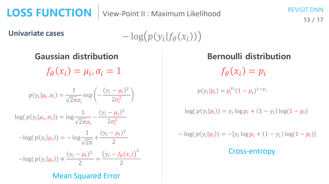
Loss Functions in the MLE perspective
Two famous loss functions, mean square error and cross-entropy error, can be derived using the MLE perspective.
 (
(