The autoencoder family

Vanilla autoencoders(AE), denoising autoencoders(DAE), variational autoencoders(VAE), and conditional variational autoencoders(CVAE) are explained in this post. Referring to the previous post on Bayesian statistics may help your understanding.

Autoencoders (AE)

Structure

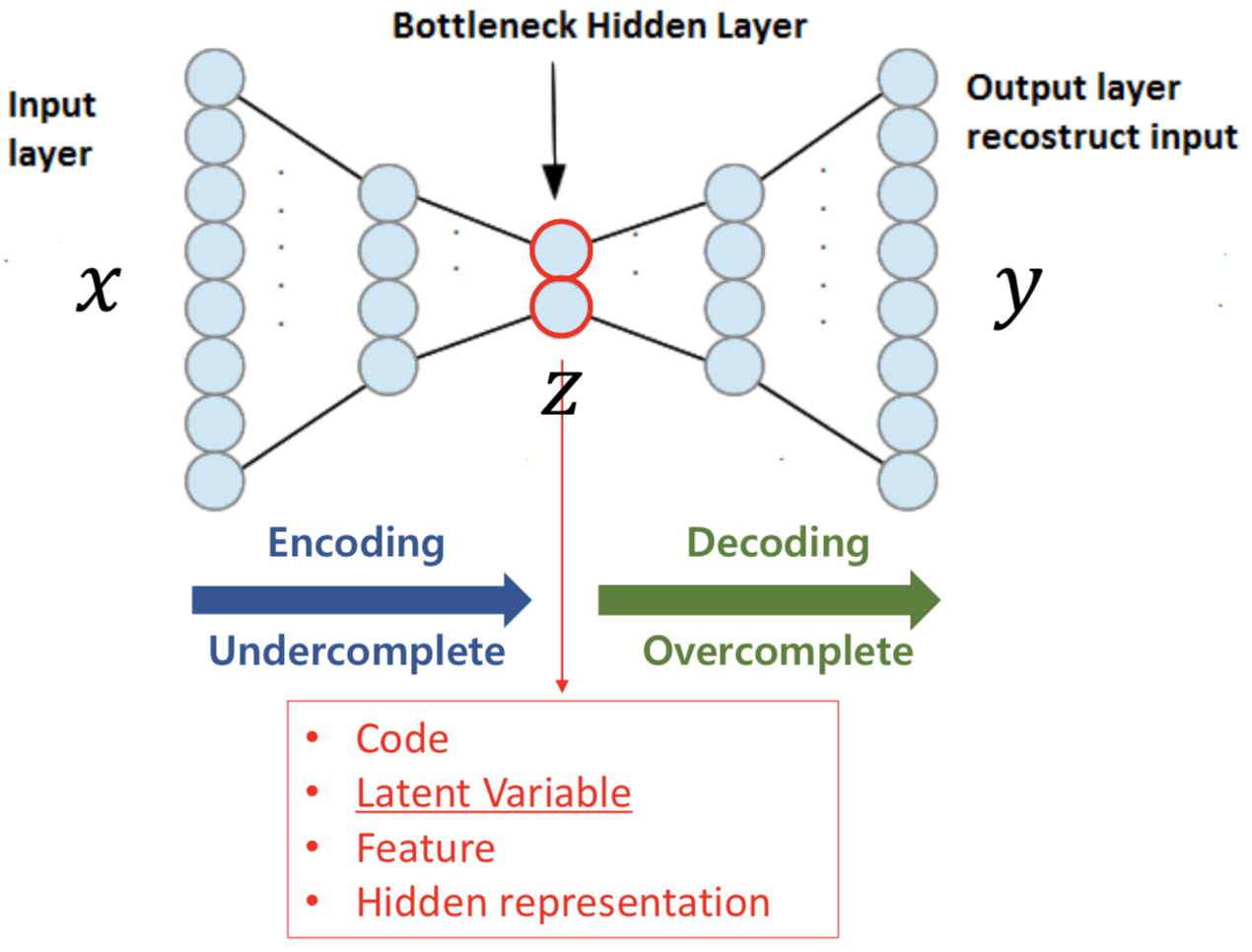
As seen in the above structure, autoencoders have the same input and output size. Ultimately, we want the output to be the same as the input. We penalize the difference of the input \(x\) and the output \(y\).

We can formulate the simplest autoencoder (with a single fully connected layer at each side) as:

\[x, y \in [0,1]^d\] \[z = h_\theta(x) = \text{sigmoid}(Wx+b) ~~~ (\theta = \{W, b\})\] \[y = g_{\theta^\prime}(z) = \text{sigmoid}(W^\prime z+b^\prime) ~~~ (\theta = \{W^\prime, b^\prime\})\]

Since we want \(x=y\), we get the following optimization problem:

\[\theta^*, \theta^{\prime *} = \underset{\theta, \theta^\prime}{\text{argmin}} \frac{1}{N} \sum_{i=1}^N l(x^{(i)}, y^{(i)})\]

The \(l(x,y)\) is the loss function, which calculates the difference between \(x\) and \(y\). We can use square error or cross-entropy, which are written as:

\[l(x, y) = \Vert x-y \Vert^2\] \[l(x, y) = - \sum_{k=1}^d [x_k \log(y_k) + (1-x_k)\log(1-y_k)]\]

We will use cross-entropy error, which we will specially denote as \(l(x, y) = L_H(x, y)\).

Statistical viewpoint

We can view this loss function in terms of expectation:

\[\theta^*, \theta^{\prime *} = \underset{\theta, \theta^\prime}{\text{argmin}} \mathbb{E}_{q^0(X)}[L_H(X, g_{\theta^\prime}(h_\theta(X)))]\]

where \(q^0(X)\) denotes the empirical distribution associated with our \(N\) training examples.

Denoising Autoencoders (DAE)

Structure

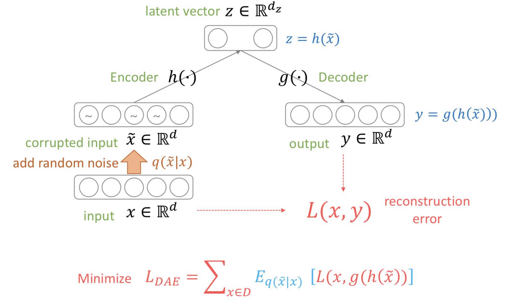
With the encoder and decoder formula the same, denoising autoencoders intentionally drop a specific portion of the pixels of the input \(x\) to zero, creating \(\tilde{x}\). Formally, we are sampling \(\tilde{x}\) from a stochastic mapping \(q_D(\tilde{x}\vert x)\). We can compute the loss between the original \(x\) and the output \(y\).

In formulating our objective function, we cannot use that of the vanilla autoencoder since now \(g_{\theta^\prime}(f_\theta(\tilde{x}))\) is a deterministic function of \(\tilde{x}\), not \(x\). Thus we need to take into account the connection between \(\tilde{x}\) and \(x\), which is \(q_D(\tilde{x}\vert x)\). Then we can write our optimization problem and expand it as:

\[\begin{aligned} \theta^*,\theta^{\prime *} &= \underset{\theta, \theta^\prime}{\text{argmin}} \mathbb{E}_{q^0(X, \tilde{X})}[L_H(X, g_{\theta^\prime}(f_\theta(\tilde{X})))]\\ &= \underset{\theta, \theta^\prime}{\text{argmin}} \frac{1}{N} \sum_{x\in D} \mathbb{E}_{q_D(\tilde{x}\vert x)}[L_H(x, g_{\theta^\prime}(f_\theta(\tilde{x})))]\\ &\approx \underset{\theta, \theta^\prime}{\text{argmin}}\frac{1}{N} \sum_{x\in D} \frac{1}{L} \sum_{i=1}^L L_H(x, g_{\theta^\prime}(f_\theta(\tilde{x}_i))) \end{aligned}\]

where \(q^0(X, \tilde{X}) = q^0(X)q_D(\tilde{X}\vert X)\). Since we cannot compute the expectation in the second line, we approximate it with the Monte Carlo technique by drawing \(L\) samples and computing their mean loss.

Variational Autoencoders (VAE)

Structure

VAEs have the same network structure with AEs; an encoder that calculates latent variable \(z\) and a decoder that generates output image \(y\). Also, we train both networks such that the output image and the input image are the same. However, their goal is what’s different. The goal of an autoencoder is to generate the best feature vector \(z\) from an image, whereas the goal of a variational autoencoder is to generate realistic images from the vector \(z\).

Also, the network structure of AEs and VAEs are not exactly the same. The encoder of an AE directly calculates the latent variable \(z\) from the input. On the other hand, the encoder of a VAE calculates the parameters of a Gaussian distribution ( \(\mu\) and \(\sigma\)), where we then sample our \(z\) from. This is true for the decoder too. AEs output the image itself, but VAE output parameters for the image pixel distribution. Let us put this more formally.

• Encoder
  Let a standard normal distribution \(p(z)\) be the prior distribution of latent variable \(z\). Given an input image \(x\), we have our encoder network calculate the posterior distribution \(p(z \vert x)\). Then we sample our latent variable \(z\) from the posterior distribution.

• Decoder
  Given a latent variable \(z\), the likelihood of our decoder outputting \(x\)(the input image) is \(p(x \vert z)\). We usually interpret this as a Multivariate Bernoulli where each pixel of the image corresponds to a dimension.

The Optimization Problem

We want to sample \(z\) from the posterior \(p(z \vert x)\), which can be expanded with the Bayes Rule.

\[p(z \vert x) = \frac{p(x \vert z)p(z)}{p(x)}\]

However \(p(x) = \int p(x \vert z ) p(z) dz\), the evidence, is intractable since we need to integrate over all possible \(z\). Thus without calculating the posterior \(p(z \vert x)\), we’ll try to approximate it with a Gaussian distribution \(q_\lambda (z \vert x)\). We call this variational inference.

Since we want the two distributions \(q_\lambda (z \vert x)\) and \(p(z \vert x)\) to be similar, we adopt the Kullback-Leibler Divergence and try to minimize it with respect to parameter \(\lambda\).

\[\begin{aligned} D_{KL}(q_\lambda(z \vert x) \vert \vert p(z \vert x)) &= \int_{-\infty}^{\infty} q_\lambda (z \vert x)\log \left( \frac{q_\lambda (z \vert x)}{p(z \vert x)} \right) dz\\ &=\mathbb{E}_q\left[ \log(q_\lambda (z \vert x)) \right] - \mathbb{E}_q \left[ \log (p(z \vert x)) \right] \\ &=\mathbb{E}_q\left[ \log(q_\lambda (z \vert x)) \right] - \mathbb{E}_q \left[ \log (p(z, x)) \right] + \log(p(x))\\ \end{aligned}\]

The problem here is that the intractable \(p(x)\) term is still present. Now let us write the above equation in terms of \(\log(p(x))\).

\[\log(p(x)) = D_{KL}(q_\lambda(z \vert x) \vert \vert p(z \vert x)) + \text{ELBO}(\lambda)\]

where

\[\text{ELBO}(\lambda) = \mathbb{E}_q \left[ \log (p(z, x)) \right] - \mathbb{E}_q\left[ \log(q_\lambda (z \vert x)) \right]\]

KL divergences are always non-negative, and we want to minimize it with respect to \(\lambda\). This is equivalent to maximizing the ELBO with respect to \(\lambda\). The abbreviation is revealed: Evidence Lower BOund. This can also be understood as maximizing the evidence \(p(x)\) since we want to maximize the probability of getting the exact input image from the output.

ELBO

Let’s inspect the \(\text{ELBO}\) term. Since no two input images share the same latent variable \(z\), we can write \(\text{ELBO}_i (\lambda)\) for a single input image \(x_i\).

\[\begin{aligned} \text{ELBO}_i (\lambda) &= \mathbb{E}_q \left[ \log (p(z, x_i)) \right] - \mathbb{E}_q\left[ \log(q_\lambda (z \vert x_i)) \right] \\ &= \int \log(p(z, x_i)) q_\lambda(z \vert x_i) dz - \int \log(q_\lambda(z \vert x_i))q_\lambda(z \vert x_i) dz \\ &= \int \log(p(x_i \vert z)p(z)) q_\lambda(z \vert x_i) dz - \int \log(q_\lambda(z \vert x_i))q_\lambda(z \vert x_i) dz \\ &= \int \log(p(x_i \vert z)) q_\lambda(z \vert x_i) dz - \int q_\lambda(z \vert x_i) \log\left(\frac{q_\lambda(z \vert x_i)}{p(z)}\right)dz \\ &= \mathbb{E}_q \left[ \log (p(x_i \vert z)) \right] - D_{KL}(q_\lambda(z \vert x_i) \vert \vert p(z)) \end{aligned}\]

Now shifting our attention back to the network structure, our encoder network calculates the parameters of \(q_\lambda(z \vert x_i)\), and our decoder network calculates the likelihood \(p(x_i \vert z)\). Thus we can rewrite the above results so that the parameters match those of the autoencoder described above.

\[\text{ELBO}_i(\phi, \theta) = \mathbb{E}_{q_\phi} \left[ \log(p_\theta(x_i \vert z)) \right] - D_{KL}(q_\phi(z \vert x_i) \vert \vert p(z))\]

Negating \(\text{ELBO}_i(\phi, \theta)\), we obtain our loss function for sample \(x_i\).

\[l_i(\phi, \theta) = -\text{ELBO}_i(\phi, \theta)\]

Thus our optimization problem becomes

\[\phi^*, \theta^* = \underset{\phi, \theta}{\text{argmin}} \sum_{i=1}^N \left[ -\mathbb{E}_{q_\phi} \left[ \log(p_\theta(x_i \vert z)) \right] + D_{KL}(q_\phi(z \vert x_i) \vert \vert p(z)) \right]\]

Understanding the loss function

\[l_i(\phi, \theta) = -\underline{\mathbb{E}_{q_\phi} \left[ \log(p_\theta(x_i \vert z)) \right]} + \underline{D_{KL}(q_\phi(z \vert x_i) \vert \vert p(z))}\]

The first underlined part (excluding the negative sign) is to be maximized. This is called the reconstruction loss: how similar the reconstructed image is to the input image. For each latent variable \(z\) we sample from the approximated posterior \(q_\phi(z \vert x_i)\), we calculate the log-likelihood of the decoder producing \(x_i\). Thus maximizing this term is equivalent to the maximum likelihood estimation.

The second term is the Kullback-Leibler Divergence between the approximated posterior \(q_\phi(z \vert x_i)\) and the prior \(p(z)\). This acts as a regularizer, forcing the approximated posterior to be similar to the prior distribution, which is a standard normal distribution.

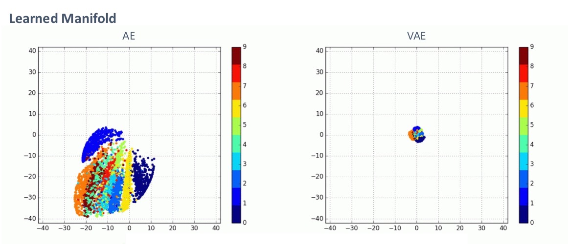
The above plots 2-dimensional latent variables of 500 test images for an AE and a VAE. As you can see, the distribution of latent variables of VAEs is close to the standard normal distribution, which is due to the regularizer. This is a virtue because, with this property, we can just easily sample a vector \(z\) from the standard normal distribution and feed it to the decoder network to generate a reasonable image. This is ideal because VAEs were intended as a generator.

Calculating the loss function

To train our VAE, we should be able to calculate the loss. Let’s start with the regularizer term.

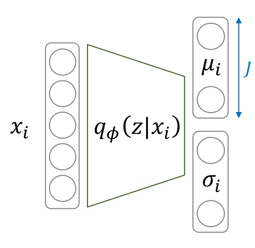
We create our encoder network such that it calculates the mean and standard deviation of \(q_\phi(z \vert x_i)\). We then sample vector \(z\) from this Multivariate Gaussian distribution: \(z \sim \mathcal{N}(\mu, \sigma^2 I)\).

The KL divergence between two normal distributions is known. We can calculate the regularizer term as:

\[D_{KL}(q_\phi(z \vert x_i) \vert \vert p(z)) = \frac{1}{2}\sum_{i=1}^J \left( \mu_{i.j}^2 + \sigma_{i,j}^2 - \log(\sigma_{i,j}^2)-1\right)\]

Now let’s look at the reconstruction loss term. To calculate the log-likelihood of our image \(\log(p_\theta(x_i \vert z))\), we should choose how to model our output. We have two choices.

1. Multivariate Bernoulli Distribution
   

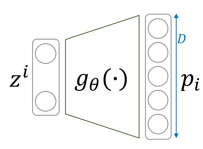
   This is often reasonable for black and white images like those from MNIST. We binarize the training and testing images with threshold 0.5. We can implement this easily with pytorch:

   image = (image >= 0.5).float()
   

   Each output of the decoder corresponds to a single pixel of the image, denoting the probability of the pixel being white. Then we can use the Bernoulli probability mass funtion \(f(x_{i,j};p_{i,j}) = p_{i,j}^{x_{i,j}} (1-p_{i,j})^{1-x_{i,j}}\) as our likelihood.

   \[\begin{aligned} \log p(x_i \vert z) &= \sum_{j=1}^D \log(p_{i,j}^{x_{i,j}} (1-p_{i,j})^{1-x_{i,j}}) \\ &= \sum_{j=1}^D \left[x_{i,j} \log(p_{i,j}) + (1-x_{i,j})\log(1-p_{i,j}) \right] \end{aligned}\]

   This is equivalent to the cross-entropy loss.

2. Multivariate Gaussian Distribution
   

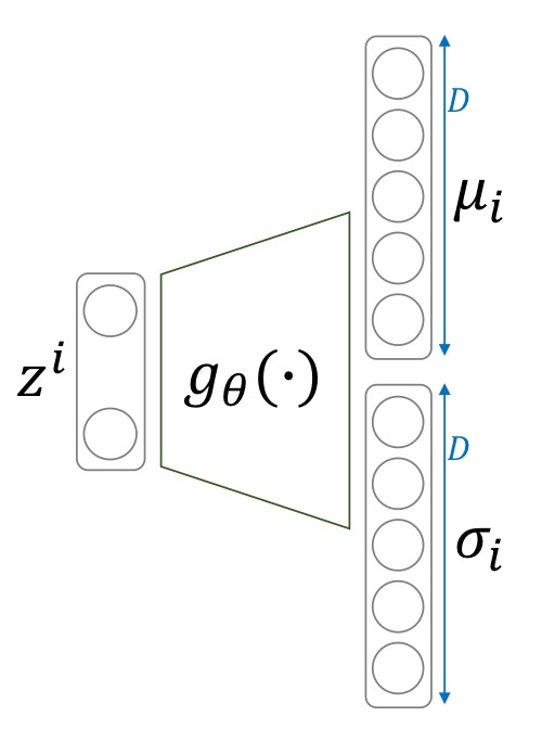
   The probability density function of a Gaussian distribution is as follows.

   \[f(x_{i,j};\mu_{i,j}, \sigma_{i,j}) = \frac{1}{\sqrt{2\pi\sigma_{i,j}^2}}e^{-\frac{(x_{i,j}-\mu_{i,j})^2}{2\sigma_{i,j}^2}}\]

   Using this in our likelihood,

   \[\log p(x_i \vert z) = -\sum_{j=1}^D \left[ \frac{1}{2}\log(\sigma_{i,j}^2)+\frac{(x_{i,j}-\mu_{i,j})^2}{2\sigma_{i,j}^2} \right]\]

   Notice that if we fix \(\sigma_{i,j} = 1\), we get the square error.

Now we’ve calculated the posterior \(p_\theta(x_i \vert z)\), we can look at the whole reconstruction loss term. Unfortunately, the expectation is difficult to compute since it takes into account every possible \(z\). So we use the Monte Carlo approximation of expectation by sampling \(L\) \(z_l\)’s from \(q_\phi(z \vert x_i)\) and take their mean log likelihood.

\[\mathbb{E}_{q_\phi} \left[ \log p_\theta(x_i \vert z) \right] \approx \frac{1}{L} \sum_{l=1}^L \log p_\theta(x_i \vert z_l )\]

For convenience, we use \(L = 1\) in implementation.

Conditional Variational Autoencoders (CVAE)

Structure

The CVAE has the same structure and loss function as the VAE, but the input data is different. Notice that in VAEs, we never used the labels of our training data. If we have labels, why don’t we use them?

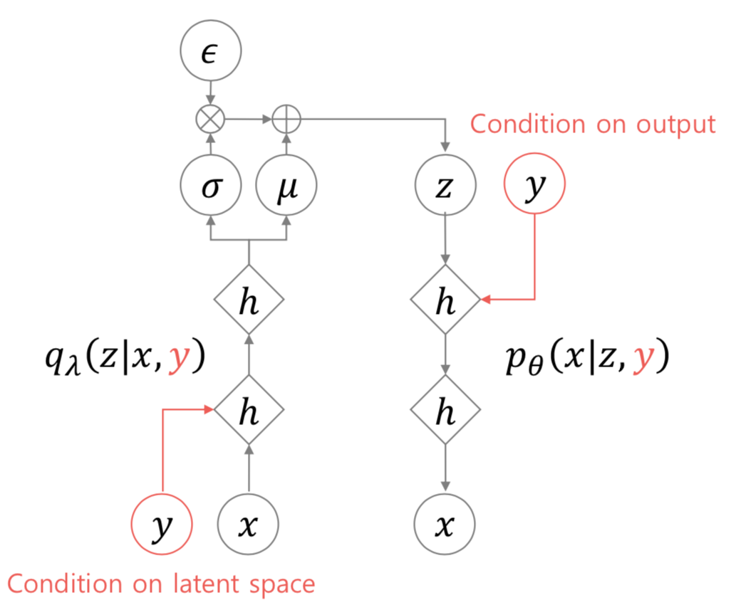
Now in conditional variational autoencoders, we concatenate the onehot labels with the input images, and also with the latent variables. Everything else is the same.

Implications

What do we get by doing this? One good thing about this is that the latent variable no longer needs to encode which label the input is. It only needs to encode its styles, or the class-invariant features of that image.

Then, we can concatenate any onehot vector to generate an image of the intended class with the specific style encoded by the latent variable.

For more images on generation, check out my repository’s README file.

Acknowledgements

• Images in this post were borrowed from the presentation by Hwalsuk Lee.

• I’ve implemented everything discussed here. Check out my GitHub repository.